## Dependencies
library(sf)
## Linking to GEOS 3.13.0, GDAL 3.8.5, PROJ 9.5.1; sf_use_s2() is TRUElibrary(raster)## Loading required package: splibrary(terra)## terra 1.8.80library(raster)
library(tmap)
library(tmaptools)
library(lidR)##
## Attaching package: 'lidR'## The following object is masked from 'package:terra':
##
## watershed## The following objects are masked from 'package:raster':
##
## projection, projection<-, wkt## The following object is masked from 'package:sp':
##
## wkt## The following object is masked from 'package:sf':
##
## st_concave_hull#library(RStoolbox)
library(ForestTools)
library(ggplot2)
library(gstat)
#install.packages("magick")
#library(magick)
library(terra)
remotes::install_github('r-tmap/tmap')## Using GitHub PAT from the git credential store.## Skipping install of 'tmap' from a github remote, the SHA1 (41111742) has not changed since last install.
## Use `force = TRUE` to force installationlibrary(rgl)
#install.packages("rgl", type = "source")#Initial plots for checking
#Burt lake raster containing Camp AGQ
dtm1 <- rast("burtlidar_2019_FEMA_19county_MI_J1277648/burtlidar_2019_FEMA_19county_MI_J1277648tR0_C0.tif")
dtm_clip <-rast("dtm_clip.tif")
# Optional: save to disk
#writeRaster(dtm1, "dtm_mosaic.tif", overwrite = TRUE)
# Plot
plot(dtm1)
plot(dtm_clip)
#If 3D is working:
#plot_dtm3d(dtm1)
#render_snapshot(filename = "burtlake_dtm_rayshader.png")
#library(rgl)

# Assuming your 3D model is already rendered with plot_3d()


#movie3d(
#  movie   = "burtlake_spin",
#  spin3d(axis = c(0, 0, 1), rpm = 6),  # very fast spin (~1 rotation per #0.5s)
# duration = 0.5,   # total animation time (seconds)
#  frames   = 16,    # number of frames to capture
#  dir      = getwd(),  # export to working directory
#  webshot  = FALSE,    # use built-in rgl capture
#  type     = "gif"     # export as GIF
#)

# Output file: "burtlake_spin.gif" in your working directory
#movie3d(
# movie = "burtlake_spin",
# spin3d(axis = c(0, 0, 1), rpm = 6), # very fast spin (~1 rotation per #0.5s)
# duration = 0.5, # total animation time (seconds)
# frames = 16, # number of frames to capture
# dir = getwd(), # export to working directory
# webshot = FALSE, # use built-in rgl capture
# type = "gif" # export as GIF
#)
# Output file: "burtlake_spin.gif" in your working directory1. SHADED DTM (HILLSHADE)
# Make sure dtm1 is in a projected CRS (it should be)
crs(dtm1)
## [1] "PROJCRS[\"NAD83(2011) / Michigan Central (ft)\",\n BASEGEOGCRS[\"NAD83(2011)\",\n DATUM[\"NAD83 (National Spatial Reference System 2011)\",\n ELLIPSOID[\"GRS 1980\",6378137,298.257222101,\n LENGTHUNIT[\"metre\",1]]],\n PRIMEM[\"Greenwich\",0,\n ANGLEUNIT[\"degree\",0.0174532925199433]],\n ID[\"EPSG\",6318]],\n CONVERSION[\"SPCS83 Michigan Central zone (international foot)\",\n METHOD[\"Lambert Conic Conformal (2SP)\",\n ID[\"EPSG\",9802]],\n PARAMETER[\"Latitude of false origin\",43.3166666666667,\n ANGLEUNIT[\"degree\",0.0174532925199433],\n ID[\"EPSG\",8821]],\n PARAMETER[\"Longitude of false origin\",-84.3666666666667,\n ANGLEUNIT[\"degree\",0.0174532925199433],\n ID[\"EPSG\",8822]],\n PARAMETER[\"Latitude of 1st standard parallel\",45.7,\n ANGLEUNIT[\"degree\",0.0174532925199433],\n ID[\"EPSG\",8823]],\n PARAMETER[\"Latitude of 2nd standard parallel\",44.1833333333333,\n ANGLEUNIT[\"degree\",0.0174532925199433],\n ID[\"EPSG\",8824]],\n PARAMETER[\"Easting at false origin\",19685039.37,\n LENGTHUNIT[\"foot\",0.3048],\n ID[\"EPSG\",8826]],\n PARAMETER[\"Northing at false origin\",0,\n LENGTHUNIT[\"foot\",0.3048],\n ID[\"EPSG\",8827]]],\n CS[Cartesian,2],\n AXIS[\"easting (X)\",east,\n ORDER[1],\n LENGTHUNIT[\"foot\",0.3048]],\n AXIS[\"northing (Y)\",north,\n ORDER[2],\n LENGTHUNIT[\"foot\",0.3048]],\n USAGE[\n SCOPE[\"Engineering survey, topographic mapping.\"],\n AREA[\"United States (USA) - Michigan - counties of Alcona; Alpena; Antrim; Arenac; Benzie; Charlevoix; Cheboygan; Clare; Crawford; Emmet; Gladwin; Grand Traverse; Iosco; Kalkaska; Lake; Leelanau; Manistee; Mason; Missaukee; Montmorency; Ogemaw; Osceola; Oscoda; Otsego; Presque Isle; Roscommon; Wexford.\"],\n BBOX[43.8,-87.06,45.92,-82.27]],\n ID[\"EPSG\",6494]]"# Compute slope and aspect in radians
slope <- terra::terrain(dtm1, "slope", unit = "radians")## |---------|---------|---------|---------|========================================= aspect <- terra::terrain(dtm1, "aspect", unit = "radians")## |---------|---------|---------|---------|========================================= # Hillshade (sun angle: 45°, direction: 315° = NW)
hs <- shade(slope, aspect, angle = 45, direction = 315)## |---------|---------|---------|---------|========================================= # 2D plot with tmap
tmap_mode("plot")## ℹ tmap modes "plot" - "view"
## ℹ toggle with `tmap::ttm()`tm_shape(hs) +
tm_raster(style = "cont") +
tm_layout(legend.outside = TRUE,
main.title = "Hillshaded DTM - Burt Lake (Camp AGQ)")##
## ── tmap v3 code detected ───────────────────────────────────────────────────────
## [v3->v4] `tm_raster()`: instead of `style = "cont"`, use col.scale =
## `tm_scale_continuous()`.[v3->v4] `tm_layout()`: use `tm_title()` instead of `tm_layout(main.title = )`SpatRaster object downsampled to 3163 by 3163 cells.
## Variable(s) "col" contains positive and negative values, so midpoint is set to 0. Set midpoint = NA to show the full range of visual values.
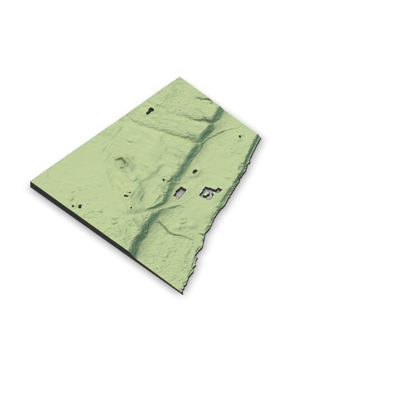
2. RAYSHADER 2D & 3D MAP
In order to get a smaller and more manageable tif, I used an in-R feature to allow me to draw an extent:
Instructions on how to clip raster in rStudio
plot(dtm1) aoi <- drawExtent() # Click and drag on the map
dtm_clip <- crop(dtm1, aoi)
plot(dtm_clip) Click and drag on the map - repeat until you’ve zoned in aoi <- drawExtent()
library(rayshader)
library(rgl)    # for interactive 3D window

# Convert SpatRaster (terra) to RasterLayer (raster package)
dtm1_raster <- raster::raster(dtm_clip)

# Convert RasterLayer to matrix for rayshader
elmat <- raster_to_matrix(dtm1_raster)

# Check dimensions
dim(elmat)
## [1] 595 487# Build a shaded relief "map" using rayshader
map <- elmat %>%
sphere_shade(texture = "imhof1", progbar = FALSE) %>%
add_water(detect_water(elmat), color = "imhof1") %>%
add_shadow(ray_shade(elmat, progbar = FALSE), 0.5) %>%
add_shadow(ambient_shade(elmat, progbar = FALSE), 0)
# 2D plot of the shaded relief
plot_map(map)
#If 3D is working:

#3D plot of the DTM with shading
#plot_3d(map, elmat,
#        zscale     = 5,          # vertical exaggeration: lower = more #stretched
#        windowsize = c(800,800))
#
#render_snapshot(filename = "burtlake_dtm.png")

#save_3dprint("burtlake_dtm.stl", maxwidth = "120mm")
#3D plot of the DTM with shading
#plot_3d(map, elmat,
# zscale = 5, # vertical exaggeration: lower = more #stretched
# windowsize = c(800,800))
#
#render_snapshot(filename = "burtlake_dtm.png")
#save_3dprint("burtlake_dtm.stl", maxwidth = "120mm")Workflow response
Using the LiDAR dataset from Burt Lake, I developed a workflow to visualize terrain features around Camp AGQ. After loading and clipping the digital terrain model (DTM) in R, I created shaded and 3D representations using packages such as terra, tmap, and rayshader. The 3D model and hillshade outputs matched what I expected for the area—gentle slopes near the shoreline and flatter terrain around the camp. Even though I haven’t studied much raster data from this location before, it was exciting to see the elevation patterns I had pictured take shape on the screen. These visualizations will be useful for my capstone project by helping me better understand local topography and how it might influence site planning or environmental factors.
Working with LiDAR data highlighted both the strengths and challenges of 3D geovisualization. The models provide an intuitive way to explore landscapes and communicate spatial ideas that 2D maps can’t fully capture, but they also require careful data management—large raster sizes and rendering limitations can slow down processing. Despite these hurdles, 3D mapping technologies are clearly advancing fast. Immersive and interactive tools like VR terrain viewers and web-based 3D maps are becoming more common in research and professional settings. I can see these methods becoming standard for analyzing and sharing spatial data in my near future.